Contents¶

deflex - flexible multi-regional energy system model for heat, power and mobility¶

++++++ multi sectoral energy system of Germany/Europe ++++++ dispatch optimisation ++++++ highly configurable and adaptable ++++++ multiple analyses functions +++++

The following README gives you a brief overview about deflex. Read the full documentation for all information.

Installation
Use example
Improve deflex
Citing deflex
Gallery
Documentation
License

Installation ¶

To run deflex you have to install the Python package and a solver:

deflex is available on PyPi and can be installed using pip install deflex.
an LP-solver is needed such as CBC (default), GLPK, Gurobi*, Cplex*
for some extra functions additional packages and are needed

* Proprietary solver

Use example ¶

Run pip install deflex[example]
Create a local directory (e.g. /home/user/deflex_examples).
Download the example scripts to this directory. There are two example. The model_example.py will explain the modelling process, the basic_analyses_example.py will show you how to analyse the results.
Read the comments of each example, execute it and modify it to your needs. Do not forget to set the my_path in the examples first.
In parallel you should read the usage guide of the documentation to get the full picture.

Improve deflex ¶

We are warmly welcoming all who want to contribute to the deflex library. This includes the following actions:

Write bug reports or comments
Improve the documentation (including typos, grammar)
Add features improve the code (open an issue first)

Citing deflex ¶

Go to the Zenodo page of deflex to find the DOI of your version. To cite all deflex versions use:

Gallery ¶

The following figures will give you a brief impression about deflex.

https://raw.githubusercontent.com/reegis/deflex/master/docs/images/model_regions.svg

Figure 1: Use one of the include regions sets or create your own one. You can also include other European countries.

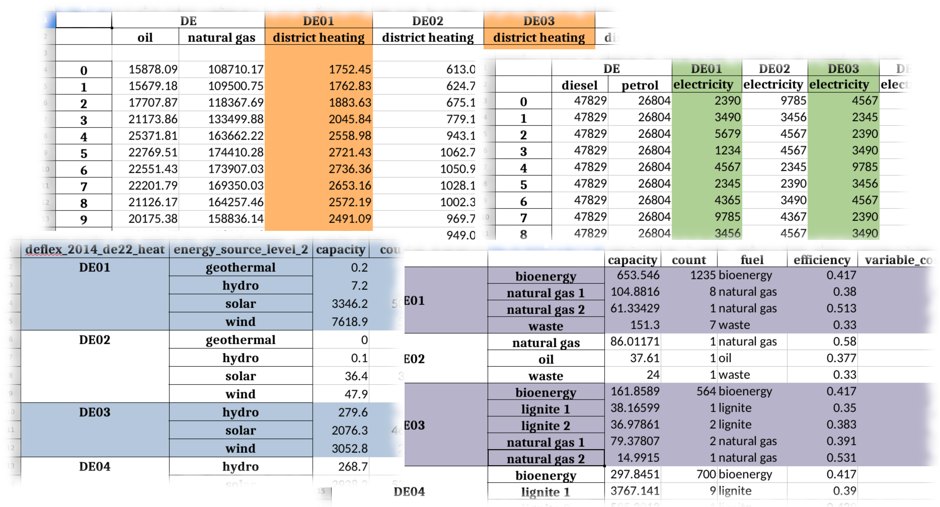
https://raw.githubusercontent.com/reegis/deflex/master/docs/images/spreadsheet_examples.png

Figure 2: The input data can be organised in spreadsheets or csv files.

https://raw.githubusercontent.com/reegis/deflex/master/docs/images/mcp.svg

Figure 3: The resulting system costs of deflex have been compared with the day-ahead prices from the Entso-e downloaded from Open Power System Data. The plot shows three different periods of the year.

https://raw.githubusercontent.com/reegis/deflex/master/docs/images/emissions.svg

Figure 4: It is also possible to get a time series of the average emissions. Furthermore, it shows the emissions of the most expensive power plant which would be replaced by an additional feed-in.

https://raw.githubusercontent.com/reegis/deflex/master/docs/images/transmission.svg

Figure 5: The following plot shows fraction of the time on which the utilisation of the power lines between the regions is more than 90% of its maximum capacity:

Documentation ¶

The full documentation of deflex is available on readthedocs.

Go to the download page to download different versions and formats (pdf, html, epub) of the documentation.

License ¶

Permission is hereby granted, free of charge, to any person obtaining a copy of this software and associated documentation files (the “Software”), to deal in the Software without restriction, including without limitation the rights to use, copy, modify, merge, publish, distribute, sublicense, and/or sell copies of the Software, and to permit persons to whom the Software is furnished to do so, subject to the following conditions:

The above copyright notice and this permission notice shall be included in all copies or substantial portions of the Software.

THE SOFTWARE IS PROVIDED “AS IS”, WITHOUT WARRANTY OF ANY KIND, EXPRESS OR IMPLIED, INCLUDING BUT NOT LIMITED TO THE WARRANTIES OF MERCHANTABILITY, FITNESS FOR A PARTICULAR PURPOSE AND NONINFRINGEMENT. IN NO EVENT SHALL THE AUTHORS OR COPYRIGHT HOLDERS BE LIABLE FOR ANY CLAIM, DAMAGES OR OTHER LIABILITY, WHETHER IN AN ACTION OF CONTRACT, TORT OR OTHERWISE, ARISING FROM, OUT OF OR IN CONNECTION WITH THE SOFTWARE OR THE USE OR OTHER DEALINGS IN THE SOFTWARE.

Installation guide¶

The deflex package is available on PyPi.

Basic version¶

The basic version of deflex can read, solve and analyse a deflex scenario. Some additional functions such as spatial operations or plots need some extra packages (see below). To install the latest stable version use:

pip install deflex

In case you have some old deflex scenario you can install the old stable phd version:

pip install https://github.com/reegis/deflex/archive/phd.zip

To get the latest features you can install the testing version:

pip install https://github.com/reegis/deflex/archive/master.zip

Installation of a solver (mandatory)¶

To solve an energy system a linear solver has to be installed. For the communication with the solver Pyomo is used. Have a look at the Pyomo docs to learn about which solvers are supported.

The default solver for deflex is the CBC solver. Go to the oemof.solph documentation to get help for the solver installation.

Additional requirements (optional)¶

The basic installation can be used to compute scenarios (csv, xls, xlsx). For some functions additional packages are needed. Some of these packages may need OS specific packages. Please see the installation guide of each package if an error occur.

To run the example with plots you need the following packages:
- matplotlib (plotting)
- pytz (time zones)
- requests (download example files)
pip install deflex[example]
To use the maps of the polygons, transmission lines etc.:
- pygeos (spatial operations)
- geopandas (maps)
pip install deflex[map]
To develop deflex:
- pytest
- sphinx
- sphinx_rtd_theme
- pygeos
- geopandas
- requests
pip install deflex[dev]

Usage guide¶

THIS CHAPTER IS WORK IN PROGRESS…

DeflexScenario
Results
- Fetch results
- Get common values from results
Parallel computing of scenarios
Input data

DeflexScenario ¶

The scenario class DeflexScenario is a central element of deflex.

All input data is stored as a dictionary in the input_data attribute of the DeflexScenario class. The keys of the dictionary are names of the data table and the values are pandas.DataFrame or pandas.Series with the data.

https://raw.githubusercontent.com/reegis/deflex/master/docs/images/deflex_scenario_class.svg

Load input data ¶

At the moment, there are two methods to populate this attribute from files:

read_csv() - read a directory with all needed csv files.
read_xlsx() - read a spread sheet in the .xlsx

To learn how to create a valid input data set see “REFERENCE”.

from deflex import scenario
sc = scenario.DeflexScenario()
sc.read_xlsx("path/to/xlsx/file.xlsx")
# OR
sc.read_csv("path/to/csv/dir")

Solve the energy system ¶

A valid input data set describes an energy system. To optimise the dispatch of the energy system a external solver is needed. By default the CBC solver is used but different solver are possible (see: solver).

The simplest way to solve a scenario is the compute() method.

sc.compute()

To use a different solver one can pass the solver parameter.

sc.compute(solver="glpk")

Store and restore the scenario ¶

The dump() method can be used to store the scenario. a solved scenario will be stored with the results. The scenario is stored in a binary format and it is not human readable.

sc.dump("path/to/store/results.dflx")

To restore the scenario use the restore_scenario function:

sc = scenario.restore_scenario("path/to/store/results.dflx")

Analyse the scenario ¶

Most analyses cannot be taken if the scenario is not solved. However, the merit order can be shown only based on the input data:

from deflex import DeflexScenario
from deflex import analyses
sc = DeflexScenario()
sc.read_xlsx("path/to/xlsx/file.xlsx")
pp = analyses.merit_order_from_scenario(sc)
ax = plt.figure(figsize=(15, 4)).add_subplot(1, 1, 1)
ax.step(pp["capacity_cum"].values, pp["costs_total"].values, where="pre")
ax.set_xlabel("Cumulative capacity [GW]")
ax.set_ylabel("Marginal costs [EUR/MWh]")
ax.set_ylim(0)
ax.set_xlim(0, pp["capacity_cum"].max())
plt.show()

With the de02_co2-price_var-costs.xlsx from the examples the code above will produce the following plot:

_images/merit_order_example_plot_simple.svg

Filling the area between the line and the x-axis with colors according the fuel of the power plant oen get the following plot:

_images/merit_order_example_plot_coloured.svg

IMPORTANT: This is just an example and not a source for the actual merit order in Germany.

Results ¶

All results are stored in ther results attribute of the Scenario class. It is a dictionary with the following keys:

main – Results of all variables

param – Input parameter

meta – Meta information and tags of the scenario

problem – Information about the linear problem such as lower bound, upper bound etc.

solver – Solver results

solution – Information about the found solution and the objective value

The deflex package provides some analyse functions as described below but it is also possible to write your own post processing. See the results chapter of the oemof.solph documentation to learn how to access the results.

Fetch results ¶

To find results file on your hard disc you can use the search_results() function. This function provides a filter parameter which can be used to filter your own meta tags. The meta attribute of the Scenario class can store these meta tags in a dictionary with the tag-name as key and the value.

meta = {
    "regions": 17,
    "heat": True,
    "tag": "value",
    }

The filter for these tags will look as follows. The values in the filter have to be strings regardless of the original type:

search_results(path=TEST_PATH, regions=["17", "21"], heat=["true"])

There is always an AND connection between all filters and an OR connectionso within a list. So The filter above will only return results with 17 or 21 regions and with the heat-tag set to true. The returning list can be used as an input parameter to load the results and get a list of results dictionaries.

my_result_files = search_results(path=my_path)
my_results = restore_results(my_result_files)

If a single file name is passed to the restore_results() function a single result will be returned, otherwise a list.

Get common values from results ¶

Common values are emissions, costs and energy of the flows. The function get_flow_results() returns a MultiIndex DataFrame with the costs, emissions and the energy of all flows. The values are absolute and specific. The specific values are divided by the power so that the specific power gives you the status (on/off).

At the moment this works only with hourly time steps. The units are as flows:

absolute emissions -> tons

specific emissions -> tons/MWh

absolute costs -> EUR

specific costs -> EUR/MWh

absolute energy -> MWh

specific energy -> –

The resulting table of the function can be stored as a .csv or .xlsx file. The input is one results dictionary:

from deflex import postprocessing as pp
from deflex.analyses import get_flow_results

my_result_files = pp.search_results(path=my_path)
my_results = pp.restore_results(my_result_files[0])
flow_results = get_flow_results(my_result)
flow_results.to_csv("/my/path/flow_results.csv")

The resulting table can be used to calculate other key values in your own functions but you can also use some ready-made functions. Follow the link to get information about each function:

calculate_market_clearing_price()

calculate_emissions_most_expensive_pp()

We are planing to add more calculations in the future. Please let us know if you have any ideas and open an issue. All these functions above are integrated in the get_key_values_from_results() function. This function takes a list of results and returns one MultiIndex DataFrame. It contains all the return values from the functions above for each scenario. The first column level contains the value names and the second level the names of the scenario. The value names are:

mcp

emissions_most_expensive_pp

The name of the scenario is taken from the name key of the meta attribute. If this key is not available you have to set it for each scenario, otherwise the function will fail. The resulting table can be stored as a .csv or .xlsx file.

from deflex import postprocessing as pp
from deflex.analyses import get_flow_results

my_result_files = pp.search_results(path=my_path)
my_results = pp.restore_results(my_result_files)
kv = get_key_values_from_results(my_results)
kv.to_csv("/my/path/key_values.csv")

If you have many scenarios, the resulting table may become quite big. Therefore, you can skip values you do not need in your resulting table. If you do need only the emissions and not the market clearing price you can exclude the mcp.

kv = get_key_values_from_results(my_results, mcp=False)

Parallel computing of scenarios ¶

For the typical work flow (creating a scenario, loading the input data, computing the scenario and storing the results) the model_scenario() function can be used.

To collect all scenarios from a given directory the function fetch_scenarios_from_dir() can be used. The function will search for .xlsx files or paths that end on _csv and cannot distinguish between a valid scenario and any .xlsx file or paths that accidentally contain _csv.

No matter how you collect a list of a scenario input data files the batch_model_scenario() function makes it easier to run each scenario and get back the relevant information about the run. It is possible to ignore exceptions so that the script will go on with the following scenarios if one scenario fails.

If you have enough memory and cpu capacity on your computer/server you can optimise your scenarios in parallel. Use the model_multi_scenarios() function for this task. You can pass a list of scenario files to this function. A cpu fraction will limit the number of processes as a fraction of the maximal available number of cpu cores. Keep in mind that for large models the memory will be the limit not the cpu capacity. If a memory error occurs the script will stop immediately. It is not possible to catch a memory error. A log-file will log all failing and successful runs.

Input data ¶

The input data is stored in the input_data attribute of the DeflexScenario class (s. DeflexScenario). It is a dictionary with the name of the data set as key and the data table itself as value (pandas.DataFrame or pandas.Series).

The input data is divided into four main topics: High-level-inputs, electricity sector, heating sector (optional) and mobility sector (optional).

Download a fictive input data example to get an idea of the structure. Then go on with the following chapter to learn everything about how to define the data for a deflex model.

Overview
High-level-input (mandatory)
Electricity sector (mandatory)
Heating sector (optional)
Mobility sector (optional)

Overview ¶

A Deflex scenario can be divided into regions. Each region must have an identifier number and be named after it as DEXX, where XX is the number. For refering the Deflex scenario as a whole (i.e. the sum of all regions) use DE only.

At the current state the distribution of fossil fuels is neglected. Therefore, in order to keep the computing time low it is recommended to define them supra-regional using DE without a number. It is still possible to define them regional for example to add a specific limit for each region.

In most cases it is also sufficient to model the fossil part of the mobility and the decentralised heating sector supra-regional. It is assumed that a gas boiler or a filling station is always supplied with enough fuel, so that the only the annual values affect the model. This does not apply to electrical heating systems or cars.

In most spread sheet software it is possible to connect cells to increase readability. These lines are interpreted correctly. In csv files the values have to appear in every cell. So the following two tables will be interpreted equally!

Connected cells

		value
DE01	F1
DE01	F2
DE02	F1

Unconnected cells

		value
DE01	F1
DE01	F2
DE02	F1

Note

NaN-values are not allowed in any table. Some columns are optional and can be left out, but if a column is present there have to be values in every row. Neutral values can be 0, 1 or inf.

General ¶

key: ‘general’, value: pandas.Series()

This table contains basic data about the scenario.

year
number of time steps
co2 price
name

INDEX

year: int, [-]: A time index will be created started with January 1, at 00:00 with the number of hours given in number of time steps.
number of time steps: int, [-]: The number of hourly time steps.
co2 price: float, [€/t]: The average price for CO₂ over the whole time period.
name: str, [-]: A name for the scenario. This name will be used to compare key values between different scenarios. Therefore, it should be unique within a group of scenarios. It does not have to be intuitive. Use the info table for a human readable description of your scenario.

Info ¶

key: ‘info’, value: pandas.Series()

On this sheet, additional information that characterizes the scenario can be added. The idea behind Info is that the user can filter stored scenarios using the search_results() function.

You can create any key-value pair which is suitable for you group of scenarios.

e.g. key: scenario_type value: foo / bar / foobar

Afterwards you can search for all scenarios where the scenario_type is foo using:

search_results(path=my_path, scenario_type=["foo"])

or with other keys and multiple values:

search_results(path=my_path, scenario_type=["foo", "bar"], my_key["v1"])

The second code line will return only files with (foo or bar) and v1.

key1
key2
key3
…	…

Commodity sources ¶

key: ‘commodity sources’, value: pandas.DataFrame()

This sheet requires data fromm all the commodities used in the scenario. The data can be provided either supra-regional under DE, regional under DEXX or as a combination of both, where some commodities are global and some are regional. Regionalised commodities are specially useful for commodities with an annual limit, for example bioenergy.

		costs	emission	annual limit
DE	F1
DE	F2
DE01	F1
DE02	F2
…	…	…	…	…

INDEX

level 0: str: Region (e.g. DE01, DE02 or DE).
level 1: str: Fuel type.

COLUMNS

costs: float, [€/MWh]: The fuel production cost.
emission: float, [t/MWh]: The fuel emission factor.
annual limit: float, [MWh]: The annual maximum energy generation (if there is one, otherwise just use inf). If the annual limit is inf in every line the column can be left out.

Data sources ¶

key: ‘data sources’, value: pandas.DataFrame()

Highly recomended. Here the type data, the source name and the url from where they were obtained can be listed. It is a free format and additional columns can be added. This table helps to make your scenario as transparent as possible.

	source	url	v1	…
cost data	Institute	http1	a1	…
pv plants	Organisation	http2	a2	…
…	…	…	…	…

Electricity sector (mandatory)¶

Electricity demand series
Power plants
Volatiles plants
Volatile series
Electricity storages
Power lines

Electricity demand series ¶

key: ‘electricity demand series’, value: pandas.DataFrame()

This sheet requires the electricity demand of the scenario as a time series. One summarised demand series for each region is enough, but it is possible to distinguish between different types. This will not have any effect on the model results but may help to distinguish the different flows in the results.

	DE01	DE02			DE03	…
	all	indsutry	buildings	rest	all	…
Time step 1						…
Time step 2						…
…	…	…	…	…	…	…

INDEX

time step: int: Number of time step. Must be uniform in all series tables.

COLUMNS

unit: [MW]

level 0: str: Region (e.g. DE01, DE02).
level 1: str: Specification of the series e.g. “all” for an overall series.

Power plants ¶

key: ‘power plants’, value: pandas.DataFrame()

The power plants will feed in the electricity bus of the region the are located. The data must be divided by region and subdivided by fuel. Each row can indicate one power plant or a group of power plants. It is possible to add additional columns for information purposes.

		capacity	fuel	efficiency	annual electricity limit	variable_cost	downtime_factor	source_region
DE01	N1
	N2
	N3
DE02	N2
DE02	N3
…	…	…	…	…	…	…	…	…

INDEX

level 0: str: Region (e.g. DE01, DE02).
level 1: str: Name, arbitrary. The combination of region and name is the unique identifier for the power plant or the group of power plants.

COLUMNS

capacity: float, [MW]: The installed capacity of the power plant or the group of power plants.
fuel: str, [-]: The used fuel of the power plant or group of power plants. The combination of source_region and fuel must exist in the commodity sources table.
efficiency: float, [-]: The average overall efficiency of the power plant or the group of power plants.
annual limit: float, [MWh]: The absolute maximum limit of produced electricity within the whole modeling period.
variable_costs: float, [€/MWh]: The variable costs per produced electricity unit.
downtime_factor: float, [-]: The time fraction of the modeling period in which the power plant or the group of power plants cannot produce electricity. The installed capacity will be reduced by this factor capacity * (1 - downtime_factor).
source_region, [-]: The source region of the fuel source. Typically this is the region of the index or DE if it is a global commodity source. The combination of source_region and fuel must exist in the commodity sources table.

Volatiles plants ¶

key: ‘volatile plants’, value: pandas.DataFrame()

Examples of volatile power plants are solar, wind, hydro, geothermal. Data must be provided divided by region and subdivided by energy source. Each row can indicate one plant or a group of plants. It is possible to add additional columns for information purposes.

		capacity
DE01	N1
	N2
DE02	N1
DE03	N1
	N3
…	…	…

INDEX

level 0: str: Region (e.g. DE01, DE02).
level 1: str: Name, arbitrary. The combination of the region and the name has to exist as a time series in the volatile series table.

COLUMNS

capacity: float, [MW]: The installed capacity of the plant.

Volatile series ¶

key: ‘volatile series’, value: pandas.DataFrame()

This sheet provides the normalised feed-in time series in MW/MW _installed. So each time series will multiplied with its installed capacity to get the absolute feed-in. Therefore, the combination of region and name has to exist in the volatile plants table.

	DE01		DE02	DE03		…
	N1	N2	N1	N1	N3	…
Time step 1						…
Time step 2						…
…	…	…	…	…	…	…

INDEX

time step: int: Number of time step. Must be uniform in all series tables.

COLUMNS

unit: [MW]

level 0: str: Region (e.g. DE01, DE02).
level 1: str: Name of the energy source specified in the previous sheet.

Electricity storages ¶

key: ‘electricity storages’, value: pandas.DataFrame()

A types of electricity storages can be defined in this table. All different storage technologies (pumped hydro, batteries, compressed air, etc) have to be entered in a general way. Each row can indicate one storage or a group of storages. It is possible to add additional columns for information purposes.

		energy content	energy inflow	charge capacity	discharge capacity	charge efficiency	discharge efficiency	loss rate
DE01	S1
	S2
DE02	S2
…	…	…	…	…	…	…	…	…

INDEX

level 0: str: Region (e.g. DE01, DE02).
level 1: str: Name, arbitrary.

COLUMNS

energy content: float, [MWh]: The maximum energy content of a storage or a group storages.
energy inflow: float, [MWh]: The amount of energy that will feed into the storage of the model period in MWh. For example a river into a pumped hydroelectric energy storage.
charge capacity: float, [MW]: Maximum capacity to charge the storage or the group of storages.
discharge capacity: float, [MW]: Maximum capacity to discharge the storage or the group of storages.
charge efficiency: float, [-]: Charging efficiency of the storage or the group of storages.
discharge efficiency: float, [-]: Discharging efficiency of the storage or the group of storages.
loss rate: float, [-]: The relative loss of the energy content of the storage. For example a loss rate or 0.01 means that the energy content of the storage will be reduced by 1% in each time step.

Power lines ¶

key: ‘power lines’, value: pandas.DataFrame()

The power lines table defines the connection between the electricity buses of each region of the scenario. There is no default connection. If no connection is defined the regions will be self-sufficient.

	capacity	efficiency
DE01-DE02
DE01-DE03
DE02-DE03
…	…	…

INDEX

Name: str: Name of the 2 connected regions separated by a dash. Define only one direction. In the model one line for each direction will be created. If both directions are defined in the table two lines for each direction will be created for the model, so that the capacity will be the sum of both lines.

COLUMNS

capacity: float, [MW]: The maximum transmission capacity of the power lines.
efficiency:float, [-]: The transmission efficiency of the power line.

Heating sector (optional)¶

Heat demand series
Decentralised heat
Chp - heat plants

Heat demand series ¶

key: ‘heat demand series’, value: pandas.DataFrame()

The heat demand can be entered regionally under DEXX or supra-regional under DE. The only type of demand that must be entered regionally is district heating. As recommendation, coal, gas, or oil demands should be treated supra-regional.

	DE01		DE02				DE
	district heating	N1	district heating	N1	N2	…	N3	N4	N5
Time step 1
Time step 2
…	…	…	…	…	…	…	…	…	…

INDEX

time step: int: Number of time step. Must be uniform in all series tables.

COLUMNS

unit: [MW]

level 0: str: Region (e.g. DE01, DE02 or DE).
level 1: str: Name. Specification of the series e.g. district heating, coal, gas. Except for district heating each combination of region and name must exist in the decentralised heat table.

Decentralised heat ¶

key: ‘decentralised heat’, value: pandas.DataFrame()

This sheet covers all heating technologies that are used to generate decentralized heat. In this context decentralised does not mean regional it represents the large group of independent heating systems. If there is no specific reason to define a heating system regional they should be defined supra-regional.

		efficiency	source	source region
DE01	N1			DE01
DE02	N1			DE02
DE02	N2			DE02
	…			…
DE	N3			DE
	N4			DE
	N5			DE

INDEX

level 0: str: Region (e.g. DE01, DE02 or DE).
level 1: str: Name, arbitrary.

COLUMNS

efficiency: float, [-]: The efficiency of the heating technology.
source: str, [-]: The source that the heating technology uses. Examples are coal, oil for commodities, but it could also be electricity in case of a heat pump. Except for electricity the combination of source and source region has to exist in the commodity sources table. The electricity source will be connected to the electricity bus of the region defined in source region.
source region: str: The region where the source comes from (see source).

Chp - heat plants ¶

key: ‘chp-heat plants’, value: pandas.DataFrame()

This sheet covers CHP and heat plants. Each plant will feed into the district heating bus of the region it it is located. The demand of district heating is defined in the heat demand series table with the name district heating. All plants of the same region with the same fuel can be defined in one row but it is also possible to divide them by additional categories such as efficiency etc.

		limit heat chp	capacity heat chp	capacity elec chp	limit hp	capacity hp	efficiency hp	efficiency heat chp	efficiency elec chp	fuel	source region
DE01	N1										DE01
	N3										DE
	N4										DE
DE02	N1										DE02
	N2										DE02
	N3										DE
	N4										DE
	N5										DE
…	…	…	…	…	…	…	…	…	…	…	…

INDEX

level 0: str: Region (e.g. DE01, DE02).
level 1: str: Name, arbitrary.

COLUMNS

limit heat chp: float, [MWh]: The absolute maximum limit of heat produced by chp within the whole modeling period.
capacity heat chp: float, [MW]: The installed heat capacity of all chp plants of the same group in the region.
capacity elect chp: float, [MW]: The installed electricity capacity of all chp plants of the same group in the region.
limit hp: float, [MWh]: The absolute maximum limit of heat produced by the heat plant within the whole modeling period.
capacity hp: float, [MW]: The installed heat capacity of all heat of the same group in the region.
efficiency hp: float, [-]: The average overall efficiency of the heat plant.
efficiency heat chp: float, [-]: The average overall heat efficiency of the chp.
efficiency elect chp: float, [-]: The average overall electricity efficiency of the chp.
fuel: str, [-]: The used fuel of the plants. The fuel name must be equal to the fuel type of the commodity sources. The combination of fuel and source region has to exist in the commodity sources table.
source_region, [-]: The source region of the fuel source. Typically this is the region of the index or DE if it is a global commodity source.

Mobility sector (optional)¶

Mobility demand series
Mobility

Mobility demand series ¶

key: ‘mobility series’, value: pandas.DataFrame()

The mobility demand can be entered regionally or supra-regional. However, it is recommended to define the mobility demand supra-regional except for electricity. The demand for electric mobility has be defined regional because it will be connected to the electricity bus of each region. The combination of region and name has to exist in the mobility table.

	DE01	DE02	…	DE
	electricity	electricity		N1
Time step 1
Time step 2
…	…	…	…	…

INDEX

time step: int: Number of time step. Must be uniform in all series tables.

COLUMNS

unit: [MW]

level 0: str: Region (e.g. DE01, DE02 or DE).
level 1: str: Specification of the series e.g. “electricity” for each region or “diesel”, “petrol” for DE.

Mobility ¶

key: ‘mobility’, value: pandas.DataFrame()

This sheet covers the technologies of the mobility sector.

		efficiency	source	source region
DE01	electricity		electricity	DE01
DE02	electricity		electricity	DE02
…
DE	N1		oil/biofuel/H2/etc	DE

INDEX

level 0: str: Region (e.g. DE01, DE02 or DE).
level 1: str: Name, arbitrary.

COLUMNS

efficiency: float, [-]: The efficiency of the fuel production. If a diesel demand is defined in the mobility demand series table the efficiency represents the efficiency of diesel production from the commodity source e.g. oil. For a biofuel demand the efficiency of the production of biofuel from biomass has to be defined.
source: str, [-]: The source that the technology uses. Except for electricity the combination of source and source region has to exist in the commodity sources table. The electricity source will be connected to the electricity bus of the region defined in source region.
source region: str, [-]: The region where the source comes from.

Reference¶

deflex.analyses module¶

Analyses of deflex.

SPDX-FileCopyrightText: 2016-2020 Uwe Krien <krien@uni-bremen.de>

SPDX-License-Identifier: MIT

deflex.analyses.check_comparision_of_merit_order(path)[source]¶

Comparison of two different ways to calculate the merit order.

Calculate the merit order from scenario
Calculate the merit order from the results

The resulting tables are not exactly the same because they will have some additional columns. The following columns should be the same.

“capacity”, “efficiency”, “fuel_emission”, “fuel”, “costs_total”, “capacity_cum”

Parameters:	path (str) – Full path of results file.

Examples

>>> from deflex import results
>>> name = "de02_no_heat_reg_merit"
>>> my_path = results.fetch_example_results(name)
>>> check_comparision_of_merit_order(my_path)
Check passed! Both merit order DataFrame tables are the same.

deflex.analyses.get_flow_results(result)[source]¶

Extract values from the flows and calculate key values.

Parameters:	result (dict) – A deflex results dictionary.
Returns:
Return type:	pandas.DataFrame

deflex.analyses.merit_order_from_results(result)[source]¶

Create a merit order from deflex results.

Parameters:	result (dict) – A deflex results dictionary.
Returns:
Return type:	pandas.DataFrame

Examples

>>> from deflex import results
>>> fn = results.fetch_example_results("de02_no_heat_reg_merit")
>>> my_results = results.restore_results(fn)
>>> a = merit_order_from_results(my_results)

deflex.analyses.merit_order_from_scenario(path, with_downtime=True, with_co2_price=True)[source]¶

Create a merit order from a deflex scenario.

TODO: Check transmission. TODO: Add volatile sources as an optional feature TODO: Check chp. Warn if chp are present. Add chp as an option TODO: Or warn if no chp are present, installed capacity might be too high

Parameters:	path (str) – Path of the directory where the csv files of the scenario are located. with_downtime (bool) – Use down time factor to reduce the installed capacity. with_co2_price (bool) – Consider the CO2 price to calculate the merit order.
Returns:
Return type:	pandas.DataFrame

Examples

>>> import os
>>> my_path = os.path.join(os.path.dirname(__file__), os.pardir, os.pardir,
...                        "tests", "data", "deflex_2014_de02_test_csv")
>>> mo1 = merit_order_from_scenario(my_path)
>>> round(mo1.capacity_cum.iloc[-1], 4)
71.9878
>>> round(mo1.capacity.sum(), 1)
71987.8
>>> round(mo1.loc[("DE01", "natural gas"), "costs_total"], 2)
59.93
>>> mo2 = merit_order_from_scenario(my_path, with_downtime=False)
>>> int(round(mo2.capacity.sum(), 0))
84225
>>> mo3 = merit_order_from_scenario(my_path, with_co2_price=False)
>>> round(mo3.loc[("DE01", "natural gas"), "costs_total"], 2)
52.87

deflex.config module¶

deflex.geometries module¶

Reegis geometry tools.

SPDX-FileCopyrightText: 2016-2019 Uwe Krien <krien@uni-bremen.de>

SPDX-License-Identifier: MIT

deflex.geometries.deflex_power_lines(rmap=None, rtype='lines')[source]¶

Parameters:	rmap (str) – Name of the deflex powerline map. rtype (str) – Type of the deflex powerline map (‘lines’, ‘labels’).

Examples

>>> my_lines=deflex_power_lines('de17')
>>> my_lines.geometry.iloc[0].geom_type
'LineString'
>>> len(my_lines)
31
>>> deflex_power_lines('de02').index[0]
'DE01-DE02'
>>> cfg.tmp_set('init', 'map', 'de21')
>>> deflex_power_lines().name
'de21'

deflex.geometries.deflex_regions(rmap=None, rtype='polygons')[source]¶

Parameters:	rmap (str) – Name of the deflex map. rtype (str) – Type of the deflex map (‘polygon’, ‘labels’).
Returns:
Return type:	GeoDataFrame

Examples

>>> my_regions=deflex_regions('de17')
>>> len(my_regions)
17
>>> my_regions.geometry.iloc[0].geom_type
'MultiPolygon'
>>> l=deflex_regions('de21', 'labels').loc['DE04', 'geometry']
>>> l.geom_type
'Point'
>>> l.x
13.2
>>> l.y
51.1
>>> cfg.tmp_set('init', 'map', 'de22')
>>> deflex_regions().name
'de22'
>>> list(deflex_regions('de02').index)
['DE01', 'DE02']

deflex.geometries.divide_off_and_onshore(regions)[source]¶

Sort regions into onshore and offshore regions. A namedtuple with two list of regions ids will be returned. Fetch the onshore and offshore attribute of the named tuple to get the list.

Parameters:	regions (GeoDataFrame) – A region set with the region id in the index.
Returns:
Return type:	named tuple

Examples

>>> reg=deflex_regions('de02')
>>> divide_off_and_onshore(reg).onshore
['DE01']
>>> reg=deflex_regions('de21')
>>> divide_off_and_onshore(reg).offshore
['DE19', 'DE20', 'DE21']

deflex.main module¶

Main script.

SPDX-FileCopyrightText: 2016-2019 Uwe Krien <krien@uni-bremen.de>

SPDX-License-Identifier: MIT

deflex.main.batch_model_scenario(path, named=True, file_type=None, ignore_errors=True)[source]¶

Model a single scenario in batch mode. By default errors will be ignored and returned together with the traceback.

Parameters:	path (str) – A valid deflex scenario. file_type (str or None) – Type of the input data. Valid values are ‘csv’, ‘excel’, None. If the input is non the path schould end on ‘csv’, ‘.xls’, ‘.xlsx’. named (bool) – If True a named tuple with the following fields will be returned ignore_errors (bool) – Set True to stop the script if an error occurs for debugging. By default errors are ignored and returned.
Returns:
Return type:	namedtuple

Examples

>>> fn = os.path.join(os.path.dirname(__file__), os.pardir, os.pardir,
...                   "tests", "data", "deflex_test_scenario.xls")
>>> r = batch_model_scenario(fn, ignore_errors=False)  # doctest: +ELLIPSIS
Welcome to the CBC MILP ...
>>> r.name
'deflex_test_scenario.xls'
>>> result_file = r.result_file
>>> os.path.basename(result_file)
'deflex_test_scenario_alpha.esys'
>>> r.trace
>>> r.return_value.year > 2019
True
>>> fn = os.path.join("wrong_file.xls")
>>> r = batch_model_scenario(fn)
>>> r.name
'wrong_file.xls'
>>> repr(r.return_value)
"FileNotFoundError(2, 'No such file or directory')"
>>> r.result_file
>>> r.trace  # doctest: +ELLIPSIS
'Traceback (most recent call last):...
>>> os.remove(result_file)

deflex.main.fetch_scenarios_from_dir(path, csv=True, xls=False)[source]¶

Search for files with an excel extension or directories ending with ‘_csv’.

By now it is not possible to distinguish between valid deflex scenarios and other excel files or directories ending with ‘csv’. Therefore, the given directory should only contain valid scenarios.

The function will not search recursively.

Parameters:	path (str) – Directory with valid deflex scenarios. csv (bool) – Search for csv directories. xls (bool) – Search for xls files.
Returns:	list
Return type:	Scenarios found in the given directory.

Examples

>>> test_data = os.path.join(os.path.dirname(__file__), os.pardir,
...                          os.pardir, "tests", "data")
>>> my_csv = fetch_scenarios_from_dir(test_data)
>>> len(my_csv)
2
>>> os.path.basename(my_csv[0])
'deflex_2014_de02_test_csv'
>>> my_excel = fetch_scenarios_from_dir(test_data, csv=False, xls=True)
>>> len(my_excel)
3
>>> os.path.basename(my_excel[0])
'deflex_2013_de02_test.xls'
>>> len(fetch_scenarios_from_dir(test_data, xls=True))
5

deflex.main.load_scenario(path, file_type=None)[source]¶

Create a deflex scenario object from file.

Parameters:	path (str) – A valid deflex scenario file. file_type (str or None) – Type of the input data. Valid values are ‘csv’, ‘excel’, None. If the input is non the path should end on ‘csv’, ‘.xls’, ‘.xlsx’ to allow auto-detection.
Returns:
Return type:	deflex.DeflexScenario

Examples

>>> fn = os.path.join(os.path.dirname(__file__), os.pardir, os.pardir,
...                   "tests", "data", "deflex_test_scenario.xls")
>>> s = load_scenario(fn, file_type="excel")
>>> type(s)
<class 'deflex.scenario_tools.DeflexScenario'>
>>> int(s.table_collection["volatile_source"]["capacity"]["DE02", "wind"])
517
>>> type(load_scenario(fn))
<class 'deflex.scenario_tools.DeflexScenario'>
>>> load_scenario(fn, file_type="csv")  # doctest: +IGNORE_EXCEPTION_DETAIL
Traceback (most recent call last):
 ...
NotADirectoryError: [Errno 20] Not a directory:

deflex.main.model_multi_scenarios(scenarios, cpu_fraction=0.2, log_file=None)[source]¶

Parameters:	scenarios (iterable) – Multiple scenarios to be modelled in parallel. cpu_fraction (float) – Fraction of available cpu cores to use for the parallel modelling. A resulting dezimal number of cores will be rounded up to an integer. log_file (str) – Filename to store the log file.

Examples

>>> fn1 = os.path.join(os.path.dirname(__file__), os.pardir, os.pardir,
...                    "tests", "data", "deflex_test_scenario.xls")
>>> fn2 = os.path.join(os.path.dirname(__file__), os.pardir, os.pardir,
...                    "tests", "data", "deflex_test_scenario_broken.xls")
>>> my_log_file = os.path.join(os.path.dirname(__file__), os.pardir,
...                            os.pardir, "tests", "data",
...                            "my_log_file.csv")
>>> my_scenarios = [fn1, fn2]
>>> model_multi_scenarios(my_scenarios, log_file=my_log_file)
>>> my_log = pd.read_csv(my_log_file, index_col=[0])
>>> good = my_log.loc["deflex_test_scenario.xls"]
>>> rv = good["return_value"]
>>> datetime.strptime(rv, "%Y-%m-%d %H:%M:%S.%f").year > 2019
True
>>> good["trace"]
nan
>>> os.path.basename(good["result_file"])
'deflex_test_scenario_alpha.esys'
>>> broken = my_log.loc["deflex_test_scenario_broken.xls"]
>>> broken["return_value"].replace("'", "")  # doctest: +ELLIPSIS
'ValueError(Missing time series for geothermal (capacity: 31.4) in DE01...
>>> broken["trace"]  # doctest: +ELLIPSIS
'Traceback (most recent call last)...
>>> broken["result_file"]
nan
>>> os.remove(my_log_file)
>>> os.remove(good["result_file"])

deflex.main.model_scenario(path=None, file_type=None, result_path=None)[source]¶

Compute a deflex scenario.

Parameters:

path (str or None) – File or directory with a valid deflex scenario. If no path is given an energy system (es) has to be passed.
file_type (str or None) – Type of the input data. Valid values are ‘csv’, ‘excel’, None. If the input is non the path schould end on ‘csv’, ‘.xls’, ‘.xlsx’.
result_path (str or None) – Path to store the output file. If None the results will be stored along with the scenarios.

Examples

>>> fn = os.path.join(os.path.dirname(__file__), os.pardir, os.pardir,
...                   "tests", "data", "deflex_test_scenario.xls")
>>> r = model_scenario(fn, file_type="excel")  # doctest: +ELLIPSIS
Welcome to the CBC MILP ...
>>> rf = os.path.join(os.path.dirname(fn), "results_cbc",
...                   "deflex_test_scenario_alpha.esys")
>>> os.remove(rf)

deflex.main.plot_scenario(path, file_type=None, image_file=None)[source]¶

Plot the graph of an energy system. If no filename is given the plot will be shown on the screen but not writen to an image file

Parameters:	path (str) – A valid deflex scenario file. file_type (str or None) – Type of the input data. Valid values are ‘csv’, ‘excel’, None. If the input is none the path should end on ‘csv’, ‘.xls’, ‘.xlsx’ to allow auto detection. image_file (str) – The image file with a valid suffix (e.g. png, pdf, svg).
Returns:	TODO
Return type:	Keep this test? It does not work without graphviz-dev and python3-dev

Examples

>>> fn = os.path.join(os.path.dirname(__file__), os.pardir, os.pardir,
...      "tests", "data", "deflex_test_scenario.xls")
>>> fn_img = os.path.join(os.path.dirname(__file__), os.pardir, os.pardir,
...                       "tests", "data", "test_es.graphml")
>>> plot_scenario(fn, "excel", fn_img)
>>> os.path.isfile(fn_img)
True
>>> os.remove(fn_img)
>>> os.path.isfile(fn_img)
False

deflex.main.stopwatch()[source]¶: Track the running time.

deflex.nodes module¶

deflex.postprocessing module¶

deflex.scenario module¶

deflex.scenario_creator module¶

deflex.tools module¶

Processing a list of power plants in Germany.

SPDX-FileCopyrightText: 2016-2019 Uwe Krien <krien@uni-bremen.de>

SPDX-License-Identifier: MIT

deflex.tools.download(fn, url)[source]¶

deflex.transmission module¶

Processing a list of power plants in Germany.

SPDX-FileCopyrightText: 2016-2019 Uwe Krien <krien@uni-bremen.de>

SPDX-License-Identifier: MIT

deflex.transmission.add_reverse_direction(df)[source]¶: Duplicate all entries of a DataFrame with a reverse index. The index must contain a dash between two sub-strings.

deflex.transmission.get_electrical_transmission_default(rmap=None, power_lines=None, both_directions=False)[source]¶

Creates a default set of transmission capacities, distance and efficiency. The map of the lines must exist in the geometries directory. The default values are infinity for the capacity, nan for the distance and 1 for the efficiency.

Parameters:	rmap (str) – The name of the transmission line map, that is part of deflex. power_lines (iterable[str]) – A list of names of transmission lines. All name must contain a dash between the id of the regions (FromRegion-ToRegion). both_directions (bool) – If True any line will be replicated in the reverse direction.
Returns:	Transmission capacity, distance and efficiency between regions
Return type:	pd.DataFrame

Examples

>>> df=get_electrical_transmission_default('de21')
>>> df.loc['DE10-DE12', 'capacity']
inf
>>> df.loc['DE10-DE12', 'distance']
nan
>>> df.loc['DE10-DE12', 'efficiency']
1.0
>>> len(df)
39
>>> len(get_electrical_transmission_default('de22'))
40
>>> len(get_electrical_transmission_default('de17'))
31
>>> len(get_electrical_transmission_default('de02'))
1
>>> my_lines=['reg1-reg2', 'reg2-reg3']
>>> df=get_electrical_transmission_default(power_lines=my_lines)
>>> df.loc['reg1-reg2', 'capacity']
inf
>>> df=get_electrical_transmission_default(power_lines=my_lines,
...                                          both_directions=True)
>>> df.loc['reg2-reg1', 'capacity']
inf

deflex.transmission.get_electrical_transmission_renpass(both_directions=False)[source]¶

Prepare the transmission capacity and distance between de21 regions from the renpass database. The original table of the reegis database is transferred to a csv file, which is part of the reegis package. As renpass is deprecated it will not change in the future. The index uses the format ‘region1-region2’. The distance is taken from centroid to centroid. By default every region pair exists only once. It is possible to get an entry in both directions if the parameter both_directions is set True.

The capacity calculation is taken from the description of the renpass package [1]. The data is taken from the renpass database [2].

This function is only valid for the original renpass region set.

Parameters:	both_directions (bool) – If True any line will be replicated in the reverse direction.
Returns:	Transmission capacity and distance between regions
Return type:	pd.DataFrame

References

[1]	Wiese, Frauke (2015). „Renewable Energy Pathways Simulation System – Open Source as an approach to meet challenges in energy modeling“. Diss. University of Flensburg. URL : https://www.reiner-lemoine-stiftung.de/pdf/dissertationen/Dissertation_Frauke_Wiese.pdf. (page 49)

[2]	Wiese, F.: Renpass - Renewable Energy Pathways Simulation System, https://github.com/fraukewiese/renpass

Examples

>>> translines=get_electrical_transmission_renpass()
>>> int(translines.loc['DE11-DE17', 'capacity'])
2506
>>> int(translines.loc['DE18-DE17', 'distance'])
119
>>> translines.loc['DE08-DE06']
capacity    7519.040402
distance     257.000000
Name: DE08-DE06, dtype: float64
>>> translines=get_electrical_transmission_renpass(both_directions=True)
>>> int(translines.loc['DE11-DE17', 'capacity'])
2506
>>> int(translines.loc['DE17-DE11', 'capacity'])
2506

deflex.transmission.get_grid_capacity(grid, plus, minus)[source]¶: Read the grid capacity from a given region pair from the renpass db.

deflex.transmission.scenario_transmission(table_collection, regions, name)[source]¶

Get power plants for the scenario year

Examples

>>> my_regions=geometries.deflex_regions(rmap="de21")  # doctest: +SKIP
>>> pp=scenario_powerplants(dict(), my_regions, 2014, "de21"
...     )  # doctest: +SKIP
>>> lines=scenario_transmission(pp, my_regions, "de21")  # doctest: +SKIP
>>> int(lines.loc["DE07-DE05", ("electrical", "capacity")]
...     )  # doctest: +SKIP
1978
>>> int(lines.loc["DE07-DE05", ("electrical", "distance")]
...     )  # doctest: +SKIP
199
>>> float(lines.loc["DE07-DE05", ("electrical", "efficiency")]
...     )  # doctest: +SKIP
0.9
>>> cfg.tmp_set("basic", "copperplate", "True")
>>> lines=scenario_transmission(pp, regions, "de21"
...     )  # doctest: +SKIP
>>> cfg.tmp_set("basic", "copperplate", "False")
>>> float(lines.loc["DE07-DE05", ("electrical", "capacity")]
...     )  # doctest: +SKIP
inf
>>> float(lines.loc["DE07-DE05", ("electrical", "distance")]
...     )  # doctest: +SKIP
nan
>>> float(lines.loc["DE07-DE05", ("electrical", "efficiency")]
...     )  # doctest: +SKIP
1.0

Module contents¶

Contributing¶

Contributions are welcome, and they are greatly appreciated! Every little bit helps, and credit will always be given.

Bug reports¶

When reporting a bug please include:

Your operating system name and version.

Any details about your local setup that might be helpful in troubleshooting.

Detailed steps to reproduce the bug.

Documentation improvements¶

deflex could always use more documentation, whether as part of the official deflex docs, in docstrings, or even on the web in blog posts, articles, and such.

Feature requests and feedback¶

The best way to send feedback is to file an issue at https://github.com/reegis/deflex/issues.

If you are proposing a feature:

Explain in detail how it would work.
Keep the scope as narrow as possible, to make it easier to implement.
Remember that this is a volunteer-driven project, and that code contributions are welcome :)

Development¶

To set up deflex for local development:

Fork deflex (look for the “Fork” button).

Clone your fork locally:

git clone git@github.com:YOURGITHUBNAME/deflex.git

Create a branch for local development:
```
git checkout -b name-of-your-bugfix-or-feature
```
Now you can make your changes locally.
When you’re done making changes run all the checks and docs builder with tox one command:
```
tox
```

Commit your changes and push your branch to GitHub:

git add .
git commit -m "Your detailed description of your changes."
git push origin name-of-your-bugfix-or-feature

Submit a pull request through the GitHub website.

Pull Request Guidelines¶

If you need some code review or feedback while you’re developing the code just make the pull request.

For merging, you should:

Include passing tests (run tox) [1].
Update documentation when there’s new API, functionality etc.
Add a note to CHANGELOG.rst about the changes.
Add yourself to AUTHORS.rst.

[1]	If you don’t have all the necessary python versions available locally you can rely on Travis - it will run the tests for each change you add in the pull request. It will be slower though …

Tips¶

To run a subset of tests:

tox -e envname -- pytest -k test_myfeature

To run all the test environments in parallel:

tox -p auto

Development¶

To run all the tests run:

tox

Note, to combine the coverage data from all the tox environments run:

Windows	set PYTEST_ADDOPTS=--cov-append tox
Other	PYTEST_ADDOPTS=--cov-append tox

Authors¶

Uwe Krien - University of Bremen

Changelog¶

0.3.0 (2021-03-25)¶

There are many API changes in the v0.3.0 release but it is planned to keep the API more stable from now on.

Layout of input data changed
Attributes und function names for adapted.
Documentation now covers all parts of the package
Examples and illustrative images were added
Code were cleaned up
Tests are more stable, test coverage increased slightly
Example data (v03) can be downloaded from the deflex OSF page.

Authors

Uwe Krien
Pedro Duran

0.2.0 (2021-01-25)¶

Move basic scenario with reegis dependency to new package
Revise structure
Add tox tests: pyflake, docs, coverage, tests, link-test, manifest, isort

Authors

Uwe Krien

Contents¶

deflex - flexible multi-regional energy system model for heat, power and mobility¶

Installation guide¶

Basic version¶

Installation of a solver (mandatory)¶

Additional requirements (optional)¶

Usage guide¶

Reference¶

deflex.analyses module¶

deflex.config module¶

deflex.geometries module¶

deflex.main module¶

deflex.nodes module¶

deflex.postprocessing module¶

deflex.scenario module¶

deflex.scenario_creator module¶

deflex.tools module¶

deflex.transmission module¶

Module contents¶

Contributing¶

Bug reports¶

Documentation improvements¶

Feature requests and feedback¶

Development¶

Pull Request Guidelines¶

Tips¶

Development¶

Authors¶

Changelog¶

0.3.0 (2021-03-25)¶

0.2.0 (2021-01-25)¶

Indices and tables¶