Usage guide

THIS CHAPTER IS WORK IN PROGRESS…

DeflexScenario

The scenario class DeflexScenario is a central element of deflex.

All input data is stored as a dictionary in the input_data attribute of the DeflexScenario class. The keys of the dictionary are names of the data table and the values are pandas.DataFrame or pandas.Series with the data.

Load input data

At the moment, there are two methods to populate this attribute from files:

• read_csv() - read a directory with all needed csv files.
• read_xlsx() - read a spread sheet in the .xlsx

To learn how to create a valid input data set see “REFERENCE”.

from deflex import scenario
sc = scenario.DeflexScenario()
sc.read_xlsx("path/to/xlsx/file.xlsx")
# OR
sc.read_csv("path/to/csv/dir")

Solve the energy system

A valid input data set describes an energy system. To optimise the dispatch of the energy system a external solver is needed. By default the CBC solver is used but different solver are possible (see: solver).

The simplest way to solve a scenario is the compute() method.

sc.compute()

To use a different solver one can pass the solver parameter.

sc.compute(solver="glpk")

Store and restore the scenario

The dump() method can be used to store the scenario. a solved scenario will be stored with the results. The scenario is stored in a binary format and it is not human readable.

sc.dump("path/to/store/results.dflx")

To restore the scenario use the restore_scenario function:

sc = scenario.restore_scenario("path/to/store/results.dflx")

Analyse the scenario

Most analyses cannot be taken if the scenario is not solved. However, the merit order can be shown only based on the input data:

from deflex import DeflexScenario
from deflex import analyses
sc = DeflexScenario()
sc.read_xlsx("path/to/xlsx/file.xlsx")
pp = analyses.merit_order_from_scenario(sc)
ax = plt.figure(figsize=(15, 4)).add_subplot(1, 1, 1)
ax.step(pp["capacity_cum"].values, pp["costs_total"].values, where="pre")
ax.set_xlabel("Cumulative capacity [GW]")
ax.set_ylabel("Marginal costs [EUR/MWh]")
ax.set_ylim(0)
ax.set_xlim(0, pp["capacity_cum"].max())
plt.show()

With the de02_co2-price_var-costs.xlsx from the examples the code above will produce the following plot:

Filling the area between the line and the x-axis with colors according the fuel of the power plant oen get the following plot:

IMPORTANT: This is just an example and not a source for the actual merit order in Germany.

Scripts

Console scripts

The console scripts can be used to model a scenario without using Python directly (Python need to be installed, though).

Get the help message by typing

deflex-compute --help

The reference can also be found here: main()

If you dumped your results you can also use postprocessing tools. Read the help message for more information by typing:

deflex-result --help

The reference can also be found here: result() See the results section for more information about the postprocessing function and classes. Not all postprocessing tools can be used with the console script.

Python scripts

For the typical work flow (creating a scenario, loading the input data, computing the scenario and storing the results) the model_scenario() function can be used.

To collect all scenarios from a given directory the function search_input_scenarios() can be used. The function will search for .xlsx files or paths that end on _csv and cannot distinguish between a valid scenario and any .xlsx file or paths that accidentally contain _csv.

No matter how you collect a list of a scenario input data files the batch_model_scenario() function makes it easier to run each scenario and get back the relevant information about the run. It is possible to ignore exceptions so that the script will go on with the following scenarios if one scenario fails.

If you have enough memory and cpu capacity on your computer/server you can optimise your scenarios in parallel. Use the model_multi_scenarios() function for this task. You can pass a list of scenario files to this function. A cpu fraction will limit the number of processes as a fraction of the maximal available number of cpu cores. Keep in mind that for large models the memory will be the limit not the cpu capacity. If a memory error occurs the script will stop immediately. It is not possible to catch a memory error. A log-file will log all failing and successful runs.

Input data

The input data is stored in the input_data attribute of the DeflexScenario class (s. DeflexScenario). It is a dictionary with the name of the data set as key and the data table itself as value (pandas.DataFrame or pandas.Series).

The input data is divided into four main topics: High-level-inputs, electricity sector, heating sector (optional) and mobility sector (optional).

Download examples (link) to get an idea of the typical structure. Then go on with the following chapter to learn everything about how to define the data of a deflex model.

Overview

A Deflex scenario can be divided into regions. Each region must have an identifier number and be named after it as DEXX, where XX is the number. For refering the Deflex scenario as a whole (i.e. the sum of all regions) use DE only.

At the current state the distribution of fossil fuels is neglected. Therefore, in order to keep the computing time low it is recommended to define them supra-regional using DE without a number. It is still possible to define them regional for example to add a specific limit for each region.

Note

The nomenclature above is the one used in the examples. It is also possible to extend it e.g. for surrounding countries (AT, FR, PL…) or to totally deviate from it. Nevertheless, it might be helpful to keep the basic idea of using the country code of the top level domain followed by a number if subregions exist or without a number. This will help other users to understand your data.

In most cases it is also sufficient to model the fossil part of the mobility and the decentralised heating sector supra-regional. It is assumed that a gas boiler or a filling station is always supplied with enough fuel, so that only the annual values affect the model. This does not apply to electrical heating systems or cars.

In most spread sheet software it is possible to connect cells to increase readability. These lines are interpreted correctly. In csv files the values have to appear in every cell. So the following two tables will be interpreted equally!

Connected cells

		value
DE01	F1
	F2
DE02	F1

Unconnected cells

		value
DE01	F1
DE01	F2
DE02	F1

Note

NaN-values are not allowed in any table. Some columns are optional and can be left out, but if a column is present there have to be values in every row. Neutral values can be 0, 1 or inf.

High-level-input (mandatory)

General

key: ‘general’, value: pandas.Series()

This table contains basic data about the scenario.

year
co2 price
number of time steps
name

INDEX

year: int, [-]

A time index will be created starting with January 1, at 00:00 with the number of hours given in number of time steps.

co2 price: float, [€/t]

The average price for CO₂ over the whole time period.

number of time steps: int, [-]

The number of hourly time steps.

name: str, [-]

A name for the scenario. This name will be used to compare key values between different scenarios. Therefore, it should be unique within a group of scenarios. It does not have to be intuitive. Use the info table for a human readable description of your scenario.

Info

key: ‘info’, value: pandas.Series()

On this sheet, additional information that characterizes the scenario can be added. The idea behind Info is that the user can filter stored scenarios using the search_dumped_scenarios() function.

You can create any key-value pair which is suitable for a group of scenarios.

e.g. key: scenario_type value: foo / bar / foobar

Afterwards you can search for all scenarios where the scenario_type is foo using search_dumped_scenarios(). See documentation and examples of this function for more details.

key1
key2
key3
…	…

Commodity sources

key: ‘commodity sources’, value: pandas.DataFrame()

This sheet requires data from all the commodities used in the scenario. The data can be provided either supra-regional under DE, regional under DEXX or as a combination of both, where some commodities are global and some are regional. Regionalised commodities are especially useful for commodities with an annual limit, for example bioenergy.

		costs	emission	annual limit
DE	F1
	F2
DE01	F1
DE02	F2
…	…	…	…	…

INDEX

level 0: str

Region (e.g. DE01, DE02 or DE).

level 1: str

Fuel type (e.g. natural gas or bionenergy).

COLUMNS

costs: float, [€/MWh]

The fuel production cost.

emission: float, [t/MWh]

The fuel emission factor.

annual limit: float, [MWh]

The annual maximum energy generation (if there is one, otherwise just use inf). If the annual limit is inf in every line the column can be left out.

Data sources

key: ‘data sources’, value: pandas.DataFrame()

Highly recomended. Here the type data, the source name and the url from where they were obtained can be listed. It is a free format and additional columns can be added. This table helps to make your scenario as transparent as possible.

	source	url	v1	…
cost data	Institute	http1	a1	…
pv plants	Organisation	http2	a2	…
…	…	…	…	…

Electricity sector (mandatory)

Electricity demand series

key: ‘electricity demand series’, value: pandas.DataFrame()

This sheet requires the electricity demand of the scenario as a time series. One summarised demand series for each region is enough, but it is possible to distinguish between different types. This will not have any effect on the model results but may help to distinguish the different flows in the results.

	DE01	DE02			DE03	…
	all	industry	buildings	rest	all	…
Time step 1						…
Time step 2						…
…	…	…	…	…	…	…

INDEX

time step: int

Number of time step. Must be uniform in all series tables.

COLUMNS

unit: [MW]

level 0: str

Region (e.g. DE01, DE02).

level 1: str

Specification of the series e.g. “all” for an overall series.

Power plants

key: ‘power plants’, value: pandas.DataFrame()

The power plants will feed in the electricity bus of the region the are located. The data must be divided by region and subdivided by fuel. Each row can indicate one power plant or a group of power plants. It is possible to add additional columns for information purposes.

		capacity	fuel	efficiency	annual electricity limit	variable_cost	downtime_factor	source_region
DE01	N1
	N2
	N3
DE02	N2
	N3
…	…	…	…	…	…	…	…	…

INDEX

level 0: str

Region (e.g. DE01, DE02).

level 1: str

Name, arbitrary. The combination of region and name is the unique identifier for the power plant or the group of power plants.

COLUMNS

capacity: float, [MW]

The installed capacity of the power plant or the group of power plants.

fuel: str, [-]

The used fuel of the power plant or group of power plants. The combination of source_region and fuel must exist in the commodity sources table.

efficiency: float, [-]

The average overall efficiency of the power plant or the group of power plants.

annual limit: float, [MWh]

The absolute maximum limit of produced electricity within the whole modeling period.

variable_costs: float, [€/MWh]

The variable costs per produced electricity unit.

downtime_factor: float, [-]

The time fraction of the modeling period in which the power plant or the group of power plants cannot produce electricity. The installed capacity will be reduced by this factor capacity * (1 - downtime_factor).

source_region, [-]

The source region of the fuel source. Typically this is the region of the index or DE if it is a global commodity source. The combination of source_region and fuel must exist in the commodity sources table.

Volatiles plants

key: ‘volatile plants’, value: pandas.DataFrame()

Examples of volatile power plants are solar, wind, hydro, geothermal. Data must be provided divided by region and subdivided by energy source. Each row can indicate one plant or a group of plants. It is possible to add additional columns for information purposes.

		capacity
DE01	N1
	N2
DE02	N1
DE03	N1
	N3
…	…	…

INDEX

level 0: str

Region (e.g. DE01, DE02).

level 1: str

Name, arbitrary. The combination of the region and the name has to exist as a time series in the volatile series table.

COLUMNS

capacity: float, [MW]

The installed capacity of the plant.

Volatile series

key: ‘volatile series’, value: pandas.DataFrame()

This sheet provides the normalised feed-in time series in MW/MW _installed. So each time series will multiplied with its installed capacity to get the absolute feed-in. Therefore, the combination of region and name has to exist in the volatile plants table.

	DE01		DE02	DE03		…
	N1	N2	N1	N1	N3	…
Time step 1						…
Time step 2						…
…	…	…	…	…	…	…

INDEX

time step: int

Number of time step. Must be uniform in all series tables.

COLUMNS

unit: [MW]

level 0: str

Region (e.g. DE01, DE02).

level 1: str

Name of the energy source specified in the previous sheet.

Power lines

key: ‘power lines’, value: pandas.DataFrame()

The power lines table defines the connection between the electricity buses of each region of the scenario. There is no default connection. If no connection is defined the regions will be self-sufficient.

	capacity	efficiency
DE01-DE02
DE01-DE03
DE02-DE03
…	…	…

INDEX

Name: str

Name of the 2 connected regions separated by a dash. Define only one direction. In the model one line for each direction will be created. If both directions are defined in the table two lines for each direction will be created for the model, so that the capacity will be the sum of both lines.

COLUMNS

capacity: float, [MW]

The maximum transmission capacity of the power lines.

efficiency:float, [-]

The transmission efficiency of the power line.

Electricity storages

key: ‘storages’, value: pandas.DataFrame()

Electricity storages is a particular case of storages (see Storages). The condition to use a storage as an electricity storage is to define electricity in the storage medium column.

Heating sector (optional)

Heat demand series

key: ‘heat demand series’, value: pandas.DataFrame()

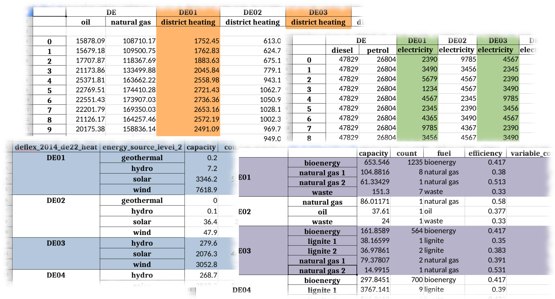
The heat demand can be entered regionally under DEXX or supra-regional under DE. The only type of demand that must be entered regionally is district heating. As recommendation, coal, gas, or oil demands should be treated supra-regional.

	DE01		DE02				DE
	district heating	N1	district heating	N1	N2	…	N3	N4	N5
Time step 1
Time step 2
…	…	…	…	…	…	…	…	…	…

INDEX

time step: int

Number of time step. Must be uniform in all series tables.

COLUMNS

unit: [MW]

level 0: str

Region (e.g. DE01, DE02 or DE).

level 1: str

Name. Specification of the series e.g. district heating, coal, gas. Except for district heating each combination of region and name must exist in the decentralised heat table.

Decentralised heat

key: ‘decentralised heat’, value: pandas.DataFrame()

This sheet covers all heating technologies that are used to generate decentralized heat. In this context decentralised does not mean regional it represents the large group of independent heating systems. If there is no specific reason to define a heating system regional they should be defined supra-regional.

		efficiency	source	source region
DE01	N1			DE01
DE02	N1			DE02
	N2			DE02
	…			…
DE	N3			DE
	N4			DE
	N5			DE

INDEX

level 0: str

Region (e.g. DE01, DE02 or DE).

level 1: str

Name, arbitrary.

COLUMNS

efficiency: float, [-]

The efficiency of the heating technology.

source: str, [-]

The source that the heating technology uses. Examples are coal, oil for commodities, but it could also be electricity in case of a heat pump. Except for electricity the combination of source and source region has to exist in the commodity sources table. The electricity source will be connected to the electricity bus of the region defined in source region.

source region: str

The region where the source comes from (see source).

Chp - heat plants

key: ‘chp-heat plants’, value: pandas.DataFrame()

This sheet covers CHP and heat plants. Each plant will feed into the district heating bus of the region it it is located. The demand of district heating is defined in the heat demand series table with the name district heating. All plants of the same region with the same fuel can be defined in one row but it is also possible to divide them by additional categories such as efficiency etc.

		limit heat chp	capacity heat chp	capacity elec chp	limit hp	capacity hp	efficiency hp	efficiency heat chp	efficiency elec chp	fuel	source region
DE01	N1										DE01
	N3										DE
	N4										DE
DE02	N1										DE02
	N2										DE02
	N3										DE
	N4										DE
	N5										DE
…	…	…	…	…	…	…	…	…	…	…	…

INDEX

level 0: str

Region (e.g. DE01, DE02).

level 1: str

Name, arbitrary.

COLUMNS

limit heat chp: float, [MWh]

The absolute maximum limit of heat produced by chp within the whole modeling period.

capacity heat chp: float, [MW]

The installed heat capacity of all chp plants of the same group in the region.

capacity elect chp: float, [MW]

The installed electricity capacity of all chp plants of the same group in the region.

limit hp: float, [MWh]

The absolute maximum limit of heat produced by the heat plant within the whole modeling period.

capacity hp: float, [MW]

The installed heat capacity of all heat of the same group in the region.

efficiency hp: float, [-]

The average overall efficiency of the heat plant.

efficiency heat chp: float, [-]

The average overall heat efficiency of the chp.

efficiency elect chp: float, [-]

The average overall electricity efficiency of the chp.

fuel: str, [-]

The used fuel of the plants. The fuel name must be equal to the fuel type of the commodity sources. The combination of fuel and source region has to exist in the commodity sources table.

source_region, [-]

The source region of the fuel source. Typically this is the region of the index or DE if it is a global commodity source.

Mobility sector (optional)

Mobility demand series

key: ‘mobility series’, value: pandas.DataFrame()

The mobility demand can be entered regionally or supra-regional. However, it is recommended to define the mobility demand supra-regional except for electricity. The demand for electric mobility has be defined regional because it will be connected to the electricity bus of each region. The combination of region and name has to exist in the mobility table.

	DE01	DE02	…	DE
	electricity	electricity		N1
Time step 1
Time step 2
…	…	…	…	…

INDEX

time step: int

Number of time step. Must be uniform in all series tables.

COLUMNS

unit: [MW]

level 0: str

Region (e.g. DE01, DE02 or DE).

level 1: str

Specification of the series e.g. “electricity” for each region or “diesel”, “petrol” for DE.

Mobility

key: ‘mobility’, value: pandas.DataFrame()

This sheet covers the technologies of the mobility sector.

		efficiency	source	source region
DE01	electricity		electricity	DE01
DE02	electricity		electricity	DE02
…
DE	N1		oil/biofuel/H2/etc	DE

INDEX

level 0: str

Region (e.g. DE01, DE02 or DE).

level 1: str

Name, arbitrary.

COLUMNS

efficiency: float, [-]

The efficiency of the fuel production. If a diesel demand is defined in the mobility demand series table the efficiency represents the efficiency of diesel production from the commodity source e.g. oil. For a biofuel demand the efficiency of the production of biofuel from biomass has to be defined.

source: str, [-]

The source that the technology uses. Except for electricity the combination of source and source region has to exist in the commodity sources table. The electricity source will be connected to the electricity bus of the region defined in source region.

source region: str, [-]

The region where the source comes from.

Other (optional)

Storages

key: ‘storages’, value: pandas.DataFrame()

Different type of storages can be defined in this table. All different storage technologies (pumped hydro, batteries, compressed air, hydrogen, etc) have to be entered in a general way. Each row can indicate one storage or a group of storages. If the storage medium is electricity, then the storage must exist in a region DEXX. Otherwise, the storage can be defined under DE. It is possible to add additional columns for information purposes.

		storage medium	energy content	energy inflow	charge capacity	discharge capacity	charge efficiency	discharge efficiency	loss rate
DE01	S1	electricity
	S2	electricity
DE02	S1	electricity
DE	S3	hydrogen
…	…	…	…	…	…	…	…	…	…

INDEX

level 0: str

Region (e.g. DE01, DE02).

level 1: str

Name, arbitrary.

COLUMNS

storage medium: str

The medium used to store energy. The storage medium must be defined in commodities, or it must be electricity.

energy content: float, [MWh]

The maximum energy content of a storage or a group storages.

energy inflow: float, [MWh]

The amount of energy that will feed into the storage of the model period in MWh. For example a river into a pumped hydroelectric energy storage.

charge capacity: float, [MW]

Maximum capacity to charge the storage or the group of storages.

discharge capacity: float, [MW]

Maximum capacity to discharge the storage or the group of storages.

charge efficiency: float, [-]

Charging efficiency of the storage or the group of storages.

discharge efficiency: float, [-]

Discharging efficiency of the storage or the group of storages.

loss rate: float, [-]

The relative loss of the energy content of the storage. For example a loss rate or 0.01 means that the energy content of the storage will be reduced by 1% in each time step.

Other converters

key: ‘other converters’, value: pandas.DataFrame()

Here, other converters than the ones already set, can be defined for linking different buses. A good example here is an electrolyser which connects electricity with hydrogen. Each converter has a source and a target bus with their respective regions. Other converter´s format is analogous to that of power plants and heat plants.

		capacity	annual limit	efficiency	variable costs	downtime factor	source	source region	target	target region
DE	electrolyser1						electricity	DE01	hydrogen	DE
DE	electrolyser2						electricity	DE02	hydrogen	DE
DE01	C1						S1	DE01	T1	DE01

INDEX

level 0: str

Region (e.g. DE01, DE02).

level 1: str

Name, arbitrary. The combination of region and name is the unique identifier for the converter or the group of converters.

COLUMNS

capacity: float, [MW]

The installed capacity of the converter or the group of converters.

annual limit: float, [MWh]

The absolute maximum limit of produced target units within the whole modeling period.

efficiency: float, [-]

The average overall efficiency of the converter or the group of converters.

variable_costs: float, [€/MWh]

The variable costs per produced target unit.

downtime_factor: float, [-]

The time fraction of the modeling period in which the converter or the group of converters cannot produce target units. The installed capacity will be reduced by this factor capacity * (1 - downtime_factor).

source: str, [-]

The source bus of the converter or group of converters. The combination of source_region and source must exist in the commodity sources table or it can be electricity with its region DEXX.

source_region, [-]

The source region of the source. Typically this is the region of the index or DE if it is a global commodity source.

target: str, [-]

The target bus of the converter or group of converters. The combination of target_region and target must exist in the commodity sources table or it can be electricity with its region DEXX.

trget_region, [-]

The target region of the target. Typically this is the region of the index or DE if it is a global commodity target.

Other demand series

key: ‘other demand series’, value: pandas.DataFrame()

Here, other demands different from electricity, heat or mobility can be entered as time series. Examples are hydrogen or synthetic fuel for the industry sector. The demands can be entered regionally under DEXX or supra-regional under DE. The format here is analogous to that of electricity, heat and mobility demand series.

	DE01		DE02		DE
	D1	D2	D1	D3	hydrogen	syn fuel
	sector 1	sector 1	sector 2	sector 3	industry	industry
Time step 1
Time step 2
…	…	…	…	…	…	…

INDEX

time step: int

Number of time step. Must be uniform in all series tables.

COLUMNS

unit: [MW]

level 0: str

Region (e.g. DE01, DE02 or DE).

level 1: str

Name. Specification of the series e.g. hydrogen, syn fuel.

level 2: str

Sector name. Specification of the series e.g. industry, LULUCF. This extra level is used to differentiate the sector in which the commodity is used, since the same commodity may be used in different sectors.

Demand response

key: ‘demand response’, value: pandas.DataFrame()

Demand response, also known as demand side management is used to represent flexibility in the demand time series. Because of that it is applied on the four different demand series. There is the option of using two different methods of demand response: the interval and the delay one. The documentation of both methods con be found in SinkDSM where the interval method corresponds to “oemof” and the delay to “DIW” method. Depending on whether the interval or delay method is used, the shift interval or delay columns must be used. Finally, there is also the option of adding a price to use this feature.

				capacity up	capacity down	method	shift interval	delay	cost up	cost down
mobility demand series	DE01	electricity	None			interval	8	0
	DE02	electricity	None			interval	8	0
	DE	oil	None			delay	0	10
electricity demand series	DE01	all	None			interval	8	0
	DE02	indsutry	None			interval	8	0
	DE02	buildings	None			interval	8	0
heat demand series	DE01	heat pump	None			interval	6	0
	DE	natural gas	None			delay	6	0
other demand series	DE	hydrogen	indsutry			delay	0	12

INDEX

level 0: str

Name of the demand serie.

level 1: str

Region (e.g. DE01, DE02 or DE)

level 2: str

Specification of the serie. The combination of region and specification of the serie has to exist in the corresponding demand serie sheet.

level 3: str

Sector name. This extra index is for when other demand series is used. If this is not the case, just write None instead.

COLUMNS

capacity up: float, [MW]

The maximum limit with respect to the demand, to which the demand can be increased.

capacity down: float, [MW]

The minimum limit with respect to the demand, to which the demand can be reduced.

method: str, [-]

The method chosen to be used.

shift interval: str, [-]

If the interval method is used, this column indicates the maximum interval that the demand can be shifted.

delay: str, [-]

If the deelay method is used, this column indicates the maximum delay that demand can be shifted.

cost up: float, [€/MWh]

The variable costs per shifted up unit

cost down: float, [€/MWh]

The variable costs per shifted down unit.

Results

All results are stored in the results attribute of the DeflexScenario class. It is a dictionary with the following keys:

• main – Results of all variables (result dictionary from oemof.solph)
• param – Input parameter
• meta – Meta information and tags of the scenario
• problem – Information about the linear problem such as lower bound, upper bound etc.
• solver – Solver results
• solution – Information about the found solution and the objective value

The deflex package provides some analyse functions as described below but it is also possible to write your own post processing based on the oemof.solph API. See the results chapter of the oemof.solph documentation to learn how to handle the results.

Restore results

Most postprocessing functions need the results dictionary of the DeflexScenario as an input. So it is possible to restore only the results dictionary. Nevertheless, also the whole DeflexScenario object can be restored.

• restore_scenario() – restore a full scenario
• restore_results() – restore only the results dictionary.

Both function need the full file name (including the path) to the dumped scenario as input parameter. If you have many dumped files onn your hard disc you can use a search function to find and filter the files.

• search_dumped_scenarios() – search dump files on your hard disc.

The output of the search function can be directly used in the restore functions from above.

Postprocessing

There are different types of postprocessing functions available. Some can be used to verify the overall behaviour of the model. This can be used for debugging but also for plausibility checks. Some can be used to calculated additional key values from the results or to prepare the results to calculate further values. Furthermore, it is possible to get the result from all model variables in the xlsx or csv format.

For most postprocessing calculations cycles can cause problems because assumptions are needed on how to deal with the cycles and it is difficult to implement all possible assumptions in the functions. Therefore it might be easier to use the basic preparation functions and write your own calculations. See below on how to identify different kind of cycles.

Custom postprocessing

For a custom post processing it is possible to filter, group and prepare the results to ones own needs. Use dictionary and list comprehensions to find the needed flows and groups. The label and the class of the nodes can be used to filter the nodes.

The keys of the results["main"] dictionary are tuples.

• FLows: (<from_node>, <to_node>)
• Components (<component>, None)
• Buses (<bus>, None)

A node can be a component or a bus. The values of the tuples are the objects or None.

Get the keys of all buses:

from oemof.solph import Bus
bus_keys = [k for k in results["Main"].keys()
            if isinstance(k[0], Bus) and k[1] is None]

Get a list of buses:

from oemof.solph import Bus
buses = [k[0] for k in results["Main"].keys()
         if isinstance(k[0], Bus) and k[1] is None]

Get a table of all flows from pv sources:

Long version:

import pandas as pd
pv_keys = [
    k
    for k in results["Main"].keys()
    if k[0].label.tag == "volatile" and k[0].label.subtag == "solar"
]
pv = {}
for pv_key in pv_keys:
    pv[dflx.label2str(pv_key[0].label)] = results["Main"][pv_key][
        "sequences"
    ]["flow"]
print(pd.DataFrame(pv))

Short version:

import pandas as pd
pv = {
    dflx.label2str(k[0].label): v["sequences"]["flow"]
    for k, v in results["Main"].items()
    if k[0].label.tag == "volatile" and k[0].label.subtag == "solar"
}
print(pd.DataFrame(pv))

For more information about the results handling also see the results chapter of the oemof.solph documentation.

The following table gives an overview over the used classes and the naming of the label of the deflex components and buses. Each label is a nametuple with the fields cat, tag, subtag and region.

Classes and labels of deflex nodes

	class	cat	tag	subtag	region
commodity bus	Bus	commodity	all	<fuel>	<region>
electricity bus	Bus	electricity	all	all	<region>
district heating bus	Bus	heat	district	all	<region>
decentralised heat bus	Bus	heat	decentralised	<fuel>	<region>
mobility bus	Bus	mobility	all	<name>	<region>
shortage source	Source	shortage	<cat of bus>	<subtag of bus>	<region>
commodity source	Source	source	commodity	<fuel>	<region>
volatile source	Source	source	volatile	<name>	<region>
power line	Transformer	line	electricity	<from region>	<to region>
mobility system	Transformer	mobility system	<name>	<fuel>	<region>
chp plant	Transformer	chp plant	<name>	<fuel>	<region>
decentralised heat system	Transformer	decentralised heat	<name>	<fuel>	<region>
heat plant	Transformer	heat plant	<name>	<fuel>	<region>
power plant	Transformer	power plant	<name>	<fuel>	<region>
other converter	Transformer	other converter	<name>	<fuel>	<region>
excess sink	Sink	excess	<cat of bus>	<subtag of bus>	<region>
electricity demand	Sink	electricity demand	electricity	<name>	<region>
district heat demand	Sink	heat demand	district	all	<region>
decentralised heat demand	Sink	heat demand	decentralised	<fuel>	<region>
mobility demand	Sink	mobility demand	mobility	<name>	<region>
other demand	Sink	other demand	other	<fuel>	<region>
storages	GenericStorage	storage	<medium>	<name>	<region>

Export all results

To export the results from all variables into the xlsx or csv format, the results can be stored in a collection of pandas.DataFrame. This collection can be stored into a file. An example for this workflow can be found in the documentation of the function:

• get_all_results() – get all results as dictionary
• dict2file() – store the dictionary into a file

Get common values from results

The following values will be returned on an hourly base:

• marginal costs [EUR/MWh]
• highest emission [tons/MWh]
• lowest emission [tons/MWh]
• marginal costs power plant [-]
• emission of marginal costs power plant [tons/MWh]

• deflex.calculate_key_values() – get key values on an hourly base

At the moment this works only with hourly time steps. This function is still work in progress and may return more key values in the future. Please write an issue on github for a discussion about further values.

Analyse flow cycles

As a directed graph is used to define an energy system. Cycles are defined as a group of successive directed flows, where the first and the last node or bus are the same. Small cycles are all storages. As this is a trivial solution of a cycle analysis storages can be excluded. Another kind of cycles are the combination of electrolysis and hydrogen power plants. Power lines will also cause cycles. Pure power line cycles can also be excluded but this will not exclude a cycle cause by an electrolysis in one region and a hydrogen power plant in another even though a power line is included in this cycle.

A cycle may not be a problem if it is not used as a cycle in the system. So it is also possible to analyse the usage of the cycle:

1. cycle – a cycle that can be used within the model
2. used cycle – a cycle in which all involved flows are used at least once.
3. suspicious cycle – a cycle in which all involved flows are used within one time step.

The following functions are available

• Cycles() – initialise a Cycle object
• cycles() – all cycles in one table per cycle
• used_cycles() – all used cycles in one table per cycle
• suspicious_cycles() – all suspicious cycles in one table per cycle
• get_suspicious_time_steps() – get the time steps in which all flows are active
• print() – print an overview of all existing cycles
• details() – print a more detailed overview of all existing cycles

Analyse the energy system graph

It is possible to convert the graph of the EnergySystem class into an nxgraph of networkx. So, it is possible to use all methods and functions of networkx associate with a directed graph (DiGraph). Furthermore, deflex provides some function to associate colors with types of nodes or with the total weight of an edge (flow). This can be used if the graph is exported to a graphml file. Such a file can be opened in e.g. yEd where the colors can be used to display the nodes and edges in the associated colors.

• DeflexGraph() – initialise a DeflexGraph object
• nxgraph() – get an DiGraph of networkx
• write() – export the graph to a graphml file
• color_edges_by_weight() – associate a color from a color map according to the total weight
• color_nodes_by_type() – associate a color by the type of the node
• color_nodes_by_substring() – associate a color by a substring of the label of the node
• group_nodes_by_type() – group all nodes of the graph by their type

Get dual variables

The dual variable is available for all buses in the energy system.

fetch_dual_results() – Get the resulta of the dual variables of all buses in one table

CHP allocation

These tool are mostly not connected to deflex but could be used in any context. The functions just implement typical allocation methods in Python code:

• allocate_fuel_deflex() – allocate the fuel with default values from a config file
• allocate_fuel() – allocate the fuel with all values defined by the user
• efficiency_method() – efficiency method
• exergy_method() – carnot or exergy method
• finnish_method() – alternative_generation or finnish method
• iea_method() – IEA method

Arrange parts of the results

This parts can be used for plots and identification of the model

• solver_results2series() – get the results returned from the external solver
• meta_results2series() – get some general and meta results
• group_buses() – group all buses by label
• get_time_index() – get the used time index
• nodes2table() – get an overview about all nodes and their total in- and outflows

Combine results and parameter

The following functions can be used for further calculations. See the examples for more information.

• fetch_converter_parameters() – get all values related to the converter
• fetch_attributes_of_commodity_sources() – get the values of the commodity sources
• get_combined_bus_balance() – combine buses in a multiregion model
• get_converter_balance() – the energy balance around converter to calculate emissions and costs

TABLE of LABELS!!!!

Plots

Deflex does not include plotting function as plotting is mostly a very individual part and there are already a lot of useful packages available. Nevertheless, deflex provides maps for the default region sets and some example on how to create spatial plots. The maps can be access using the following functions.

• deflex_geo() – Get the default maps of deflex
• divide_off_and_onshore() – distinguish offshore and onshore regions in a given map

General tools

Solph and deflex use logging messages to give a feedback from the running program, so deflex provides an easy function to activate the logger on the INFO level:

• use_logging()

Some functions does not return a table but a set of table. To store these set of tables in a xlsx-map or a collection of csv-files the following function can be used.

• dict2file()